Optimizing Stan code for a user-provided Gamma model
In [3]:
%load_ext autoreload
%autoreload 2
%matplotlib inline
import random
random.seed(1100038344)
import survivalstan
import numpy as np
import pandas as pd
from stancache import stancache
from matplotlib import pyplot as plt
The autoreload extension is already loaded. To reload it, use:
  %reload_ext autoreload
/home/jacquelineburos/miniconda3/envs/python3/lib/python3.5/site-packages/Cython/Distutils/old_build_ext.py:30: UserWarning: Cython.Distutils.old_build_ext does not properly handle dependencies and is deprecated.
  "Cython.Distutils.old_build_ext does not properly handle dependencies "
/home/jacquelineburos/.local/lib/python3.5/site-packages/IPython/html.py:14: ShimWarning: The `IPython.html` package has been deprecated. You should import from `notebook` instead. `IPython.html.widgets` has moved to `ipywidgets`.
  "`IPython.html.widgets` has moved to `ipywidgets`.", ShimWarning)
INFO:stancache.seed:Setting seed to 1245502385
Simulate survival data
In order to demonstrate the use of this model, we will first simulate
some survival data using survivalstan.sim.sim_data_exp_correlated.
As the name implies, this function simulates data assuming a constant
hazard throughout the follow-up time period, which is consistent with
the Exponential survival function.
This function includes two simulated covariates by default (age and
sex). We also simulate a situation where hazard is a function of the
simulated value for sex.
We also center the age variable since this will make it easier to
interpret estimates of the baseline hazard.
In [4]:
d = stancache.cached(
    survivalstan.sim.sim_data_exp_correlated,
    N=100,
    censor_time=20,
    rate_form='1 + sex',
    rate_coefs=[-3, 0.5],
)
d['age_centered'] = d['age'] - d['age'].mean()
INFO:stancache.stancache:sim_data_exp_correlated: cache_filename set to sim_data_exp_correlated.cached.N_100.censor_time_20.rate_coefs_54462717316.rate_form_1 + sex.pkl
INFO:stancache.stancache:sim_data_exp_correlated: Loading result from cache
*Aside: In order to make this a more reproducible example, this code is
using a file-caching function stancache.cached to wrap a function
call to survivalstan.sim.sim_data_exp_correlated. *
Explore simulated data
Here is what these data look like - this is per-subject or
time-to-event form:
In [5]:
d.head()
Out[5]:
| age | sex | rate | true_t | t | event | index | age_centered | |
|---|---|---|---|---|---|---|---|---|
| 0 | 59 | male | 0.082085 | 20.948771 | 20.000000 | False | 0 | 4.18 |
| 1 | 58 | male | 0.082085 | 12.827519 | 12.827519 | True | 1 | 3.18 |
| 2 | 61 | female | 0.049787 | 27.018886 | 20.000000 | False | 2 | 6.18 |
| 3 | 57 | female | 0.049787 | 62.220296 | 20.000000 | False | 3 | 2.18 |
| 4 | 55 | male | 0.082085 | 10.462045 | 10.462045 | True | 4 | 0.18 |
It’s not that obvious from the field names, but in this example “subjects” are indexed by the field ``index``.
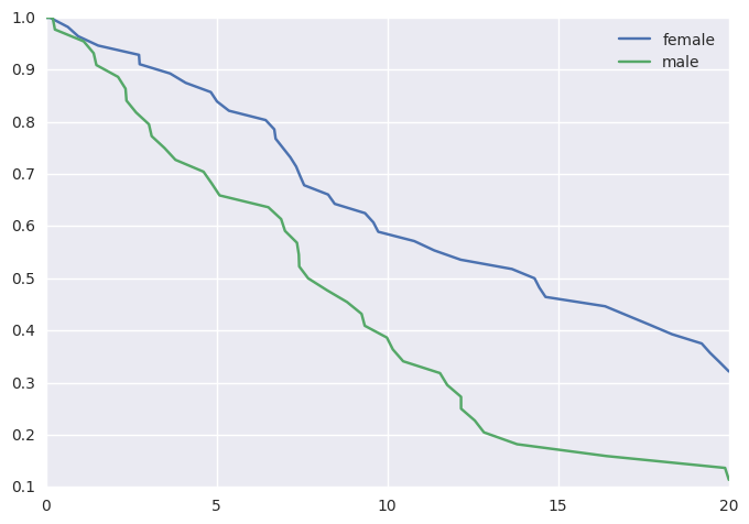
We can plot these data using lifelines, or the rudimentary plotting
functions provided by survivalstan.
In [6]:
survivalstan.utils.plot_observed_survival(df=d[d['sex']=='female'], event_col='event', time_col='t', label='female')
survivalstan.utils.plot_observed_survival(df=d[d['sex']=='male'], event_col='event', time_col='t', label='male')
plt.legend()
Out[6]:
<matplotlib.legend.Legend at 0x7f64d8063978>
model1: original spec
In [7]:
model_code = '''
functions {
  // Defines the log survival
  vector log_S (vector t, real shape, vector rate) {
    vector[num_elements(t)] log_S;
    for (i in 1:num_elements(t)) {
      log_S[i] = gamma_lccdf(t[i]|shape,rate[i]);
    }
    return log_S;
  }

  // Defines the log hazard
  vector log_h (vector t, real shape, vector rate) {
    vector[num_elements(t)] log_h;
    vector[num_elements(t)] ls;
    ls = log_S(t,shape,rate);
    for (i in 1:num_elements(t)) {
      log_h[i] = gamma_lpdf(t[i]|shape,rate[i]) - ls[i];
    }
    return log_h;
  }

  // Defines the sampling distribution
  real surv_gamma_lpdf (vector t, vector d, real shape, vector rate) {
    vector[num_elements(t)] log_lik;
    real prob;
    log_lik = d .* log_h(t,shape,rate) + log_S(t,shape,rate);
    prob = sum(log_lik);
    return prob;
  }
}

data {
  int N;                            // number of observations
  vector<lower=0>[N] y;             // observed times
  vector<lower=0,upper=1>[N] event;     // censoring indicator (1=observed, 0=censored)
  int M;                            // number of covariates
  matrix[N, M] x;                    // matrix of covariates (with n rows and H columns)
}

parameters {
  vector[M] beta;         // Coefficients in the linear predictor (including intercept)
  real<lower=0> alpha;    // shape parameter
}

transformed parameters {
  vector[N] linpred;
  vector[N] mu;
  linpred = x*beta;
  for (i in 1:N) {
    mu[i] = exp(linpred[i]);
  }
}

model {
  alpha ~ gamma(0.01,0.01);
  beta ~ normal(0,5);
  y ~ surv_gamma(event, alpha, mu);
}
'''
Now, we are ready to fit our model using
survivalstan.fit_stan_survival_model.
We pass a few parameters to the fit function, many of which are required. See ?survivalstan.fit_stan_survival_model for details.
Similar to what we did above, we are asking survivalstan to cache
this model fit object. See
stancache for more details on
how this works. Also, if you didn’t want to use the cache, you could
omit the parameter FIT_FUN and survivalstan would use the
standard pystan functionality.
In [8]:
testfit = survivalstan.fit_stan_survival_model(
    model_cohort = 'model 1',
    model_code = model_code,
    df = d,
    time_col = 't',
    event_col = 'event',
    formula = '~ age_centered + sex',
    iter = 5000,
    chains = 4,
    seed = 9001,
    FIT_FUN = stancache.cached_stan_fit,
    drop_intercept = False,
    )
INFO:stancache.stancache:Step 1: Get compiled model code, possibly from cache
INFO:stancache.stancache:StanModel: cache_filename set to anon_model.cython_0_25_1.model_code_14429915565770599621.pystan_2_12_0_0.stanmodel.pkl
INFO:stancache.stancache:StanModel: Loading result from cache
INFO:stancache.stancache:Step 2: Get posterior draws from model, possibly from cache
INFO:stancache.stancache:sampling: cache_filename set to anon_model.cython_0_25_1.model_code_14429915565770599621.pystan_2_12_0_0.stanfit.chains_4.data_25476010973.iter_5000.seed_9001.pkl
INFO:stancache.stancache:sampling: Loading result from cache
In [9]:
# 0:00:40.518775 elapsed
In [10]:
survivalstan.utils.print_stan_summary([testfit], pars=['lp__', 'alpha', 'beta'])
               mean   se_mean        sd        2.5%         50%       97.5%      Rhat
lp__    -278.113380  0.021718  1.358348 -281.579969 -277.815032 -276.424942  1.000465
alpha      1.220129  0.002561  0.170488    0.913076    1.209632    1.581949  1.000245
beta[0]   -2.703902  0.003699  0.226779   -3.173168   -2.695839   -2.275841  1.000271
beta[1]    0.608266  0.002897  0.199169    0.221442    0.606373    1.003776  1.000226
beta[2]    0.006018  0.000183  0.014844   -0.023068    0.005959    0.035536  1.000075
model2: alternate version of surv_gamma_lpdf
In [11]:
model_code2 = '''
functions {
  // Defines the log survival
  real surv_gamma_lpdf (vector t, vector d, real shape, vector rate) {
    vector[num_elements(t)] log_lik;
    real prob;
    for (i in 1:num_elements(t)) {
      log_lik[i] = d[i] * (gamma_lpdf(t[i]|shape,rate[i]) - gamma_lccdf(t[i]|shape,rate[i]))
                      + gamma_lccdf(t[i]|shape,rate[i]);
    }
    prob = sum(log_lik);
    return prob;
  }
}
data {
  int N;                            // number of observations
  vector<lower=0>[N] y;             // observed times
  vector<lower=0,upper=1>[N] event;     // censoring indicator (1=observed, 0=censored)
  int M;                            // number of covariates
  matrix[N, M] x;                    // matrix of covariates (with n rows and H columns)
}
parameters {
  vector[M] beta;         // Coefficients in the linear predictor (including intercept)
  real<lower=0> alpha;    // shape parameter
}
transformed parameters {
  vector<lower=0>[N] mu;
  {
      vector[N] linpred;
      linpred = x*beta;
      mu = exp(linpred);
  }
}

model {
  alpha ~ gamma(0.01,0.01);
  beta ~ normal(0,5);
  y ~ surv_gamma(event, alpha, mu);
}
'''
In [12]:
testfit2 = survivalstan.fit_stan_survival_model(
    model_cohort = 'model 2',
    model_code = model_code2,
    df = d,
    time_col = 't',
    event_col = 'event',
    formula = '~ age_centered + sex',
    iter = 5000,
    chains = 4,
    seed = 9001,
    FIT_FUN = stancache.cached_stan_fit,
    drop_intercept = False,
    )
INFO:stancache.stancache:Step 1: Get compiled model code, possibly from cache
INFO:stancache.stancache:StanModel: cache_filename set to anon_model.cython_0_25_1.model_code_9177012762674257483.pystan_2_12_0_0.stanmodel.pkl
INFO:stancache.stancache:StanModel: Loading result from cache
INFO:stancache.stancache:Step 2: Get posterior draws from model, possibly from cache
INFO:stancache.stancache:sampling: cache_filename set to anon_model.cython_0_25_1.model_code_9177012762674257483.pystan_2_12_0_0.stanfit.chains_4.data_25476010973.iter_5000.seed_9001.pkl
INFO:stancache.stancache:sampling: Loading result from cache
In [13]:
# 0:00:21.081723 elapsed
In [14]:
survivalstan.utils.print_stan_summary([testfit2], pars=['lp__', 'alpha', 'beta'])
               mean   se_mean        sd        2.5%         50%       97.5%      Rhat
lp__    -278.122019  0.022342  1.367441 -281.523430 -277.808097 -276.440635  1.001051
alpha      1.218976  0.002590  0.171529    0.906313    1.208893    1.586105  1.000714
beta[0]   -2.704073  0.003788  0.228848   -3.187193   -2.693108   -2.287256  1.000886
beta[1]    0.604867  0.002814  0.201056    0.208092    0.605508    0.993031  1.000143
beta[2]    0.006629  0.000188  0.014733   -0.021872    0.006506    0.036200  1.000063
model3: use log_mix inside surv_gamma_lpdf
In [15]:
model_code3 = '''
functions {
  // Defines the log survival
  real surv_gamma_lpdf (vector t, vector d, real shape, vector rate) {
    vector[num_elements(t)] log_lik;
    real prob;
    for (i in 1:num_elements(t)) {
      log_lik[i] = log_mix(d[i], gamma_lpdf(t[i]|shape,rate[i]), gamma_lccdf(t[i]|shape,rate[i]));
    }
    prob = sum(log_lik);
    return prob;
  }
}
data {
  int N;                            // number of observations
  vector<lower=0>[N] y;             // observed times
  vector<lower=0,upper=1>[N] event; // censoring indicator (1=observed, 0=censored)
  int M;                            // number of covariates
  matrix[N, M] x;                   // matrix of covariates (with n rows and H columns)
}
parameters {
  vector[M] beta;         // Coefficients in the linear predictor (including intercept)
  real<lower=0> alpha;    // shape parameter
}
transformed parameters {
  vector[N] linpred;
  vector[N] mu;
  linpred = x*beta;
  mu = exp(linpred);
}

model {
  alpha ~ gamma(0.01,0.01);
  beta ~ normal(0,5);
  y ~ surv_gamma(event, alpha, mu);
}
'''
In [16]:
testfit3 = survivalstan.fit_stan_survival_model(
    model_cohort = 'model 3',
    model_code = model_code3,
    df = d,
    time_col = 't',
    event_col = 'event',
    formula = '~ age_centered + sex',
    iter = 5000,
    chains = 4,
    seed = 9001,
    FIT_FUN = stancache.cached_stan_fit,
    drop_intercept = False,
    )
INFO:stancache.stancache:Step 1: Get compiled model code, possibly from cache
INFO:stancache.stancache:StanModel: cache_filename set to anon_model.cython_0_25_1.model_code_1293841621968646714.pystan_2_12_0_0.stanmodel.pkl
INFO:stancache.stancache:StanModel: Loading result from cache
INFO:stancache.stancache:Step 2: Get posterior draws from model, possibly from cache
INFO:stancache.stancache:sampling: cache_filename set to anon_model.cython_0_25_1.model_code_1293841621968646714.pystan_2_12_0_0.stanfit.chains_4.data_25476010973.iter_5000.seed_9001.pkl
INFO:stancache.stancache:sampling: Loading result from cache
In [17]:
#0:00:20.284146 elapsed
In [18]:
survivalstan.utils.print_stan_summary([testfit3], pars=['lp__', 'alpha', 'beta'])
               mean   se_mean        sd        2.5%         50%       97.5%      Rhat
lp__    -278.092768  0.021055  1.344719 -281.491359 -277.783232 -276.425885  1.000812
alpha      1.216429  0.002640  0.166944    0.905732    1.207800    1.576275  1.000432
beta[0]   -2.708385  0.003770  0.220966   -3.173480   -2.697460   -2.307317  1.000622
beta[1]    0.609834  0.002799  0.199563    0.223234    0.609396    1.008451  1.000295
beta[2]    0.006028  0.000180  0.014812   -0.022443    0.006036    0.036197  1.000265
model4: vectorize surv_gamma_lpdf
In [40]:
model_code4 = '''
functions {
    int count_value(vector a, real val) {
        int s;
        s = 0;
        for (i in 1:num_elements(a))
            if (a[i] == val)
                s = s + 1;
        return s;
    }

  // Defines the log survival
  real surv_gamma_lpdf (vector t, vector d, real shape, vector rate, int num_cens, int num_obs) {
    vector[2] log_lik;
    int idx_obs[num_obs];
    int idx_cens[num_cens];
    real prob;
    int i_cens;
    int i_obs;
    i_cens = 1;
    i_obs = 1;
    for (i in 1:num_elements(t)) {
        if (d[i] == 1) {
            idx_obs[i_obs] = i;
            i_obs = i_obs+1;
        }
        else {
            idx_cens[i_cens] = i;
            i_cens = i_cens+1;
        }
    }
    print(idx_obs);
    log_lik[1] = gamma_lpdf(t[idx_obs] | shape, rate[idx_obs]);
    log_lik[2] = gamma_lccdf(t[idx_cens] | shape, rate[idx_cens]);
    prob = sum(log_lik);
    return prob;
  }
}
data {
  int N;                            // number of observations
  vector<lower=0>[N] y;             // observed times
  vector<lower=0,upper=1>[N] event; // censoring indicator (1=observed, 0=censored)
  int M;                            // number of covariates
  matrix[N, M] x;                   // matrix of covariates (with n rows and H columns)
}
transformed data {
  int num_cens;
  int num_obs;
  num_obs = count_value(event, 1);
  num_cens = N - num_obs;
}
parameters {
  vector[M] beta;         // Coefficients in the linear predictor (including intercept)
  real<lower=0> alpha;    // shape parameter
}
transformed parameters {
  vector[N] linpred;
  vector[N] mu;
  linpred = x*beta;
  mu = exp(linpred);
}
model {
  alpha ~ gamma(0.01,0.01);
  beta ~ normal(0,5);
  y ~ surv_gamma(event, alpha, mu, num_cens, num_obs);
}
'''
In [41]:
testfit4 = survivalstan.fit_stan_survival_model(
    model_cohort = 'model 4',
    model_code = model_code4,
    df = d,
    time_col = 't',
    event_col = 'event',
    formula = '~ age_centered + sex',
    iter = 5000,
    chains = 4,
    seed = 9001,
    FIT_FUN = stancache.cached_stan_fit,
    drop_intercept = False,
    )
INFO:stancache.stancache:Step 1: Get compiled model code, possibly from cache
INFO:stancache.stancache:StanModel: cache_filename set to anon_model.cython_0_25_1.model_code_16881928540873162731.pystan_2_12_0_0.stanmodel.pkl
INFO:stancache.stancache:StanModel: Starting execution
INFO:pystan:COMPILING THE C++ CODE FOR MODEL anon_model_b18a6495e568fcff90662e16a3d2aa85 NOW.
INFO:stancache.stancache:StanModel: Execution completed (0:01:09.439292 elapsed)
INFO:stancache.stancache:StanModel: Saving results to cache
INFO:stancache.stancache:Step 2: Get posterior draws from model, possibly from cache
INFO:stancache.stancache:sampling: cache_filename set to anon_model.cython_0_25_1.model_code_16881928540873162731.pystan_2_12_0_0.stanfit.chains_4.data_25476010973.iter_5000.seed_9001.pkl
INFO:stancache.stancache:sampling: Starting execution
INFO:stancache.stancache:sampling: Execution completed (0:00:06.245552 elapsed)
INFO:stancache.stancache:sampling: Saving results to cache
/home/jacquelineburos/miniconda3/envs/python3/lib/python3.5/site-packages/stancache/stancache.py:284: UserWarning: Pickling fit objects is an experimental feature!
The relevant StanModel instance must be pickled along with this fit object.
When unpickling the StanModel must be unpickled first.
  pickle.dump(res, open(cache_filepath, 'wb'), pickle.HIGHEST_PROTOCOL)
In [42]:
# 0:00:06.245552 elapsed
In [43]:
survivalstan.utils.print_stan_summary([testfit4], pars=['lp__', 'alpha', 'beta'])
               mean   se_mean        sd        2.5%         50%       97.5%      Rhat
lp__    -278.097416  0.020380  1.353386 -281.543138 -277.782205 -276.445123  0.999867
alpha      1.216149  0.002525  0.169578    0.913312    1.206908    1.574024  1.000702
beta[0]   -2.708518  0.003627  0.228658   -3.188661   -2.700493   -2.278788  1.000723
beta[1]    0.610593  0.002824  0.201974    0.224438    0.607700    1.030164  1.000744
beta[2]    0.006211  0.000171  0.014493   -0.022229    0.006113    0.035095  1.000222
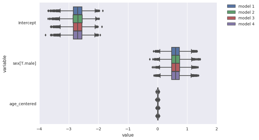
compare coefficient estimates for each model spec
In [44]:
survivalstan.utils.plot_coefs([testfit, testfit2, testfit3, testfit4])
In [ ]: